
Problem description
We have embedded devices periodically sending us data. We want to be alerted as early as possible when a device stops sending data.
A very simple approach is to take the time difference of the last few times a device sent data and calculate the average. When we know a device sends data roughly every 15 minutes, we can easily trigger an alarm if no data arrived for that time.
The above approach assumes devices send data with the same period always. However, that is unfortunately not true for all. We have found devices which never send data during the night. Or devices which stop sending every afternoon, presumably because their GSM internet connection becomes disturbed.
Idea
Since we are still talking about periodic events, one could see their occurrence as a combination of signals with different frequency. For example, the data sending behavior of a device which is not sending during the night could be modelled as a 15-minute sending frequency combined with a 24-hour sending frequency.
This is exactly what the Discrete Fourier Tranformation (DFT) is for: It transforms a signal into the frequency domain, describing it as a combination of signals with different frequencies. The idea is that by first calculating the frequency components and then doing the inverse DFT, meaning to transform these back to the time-domain, we should be able to predict when the next data sending from a device should occur.
A good description of the DFT can be found here: https://www.nayuki.io/page/how-to-implement-the-discrete-fourier-transform. Usually the DFT is not implemented straight-forward because that would be rather inefficient. Instead, optimized versions known as Fast Fourier Transformation (FFT) are used.
Getting test data
To have some real-world data to test with, we get the list of data transfers from our MongoDB:
import numpy as np
import matplotlib.pyplot as plt

# get real data from MongoDB
from pymongo import MongoClient
client = MongoClient("localhost:27017",
                     username="abc", password="xxx")

db = client["DATABASE-1_0_0"]
coll = db["datalogger-newdata"]
mongoresults = list(coll.find({"client_id":"de_alsdorf"})
                    .sort("lastCycleTime",1))

# list of timestamps of every run that found new data
runs = []
for m in mongoresults:
    runs.append(m["lastCycleTime"])
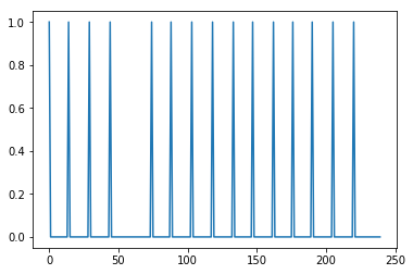
Next, we build a big minute array with 1.0-values just at these minutes in which we received new data:
time = [1]
prevrun = runs[0]
for run in runs:
    time.extend(np.zeros((run-prevrun).seconds // 60))
    time[len(time)-1] = 1.0
    prevrun = run
Let’s visualize the first 4 hours:
plt.plot(time[:240])
Perform FFT
For these tests we use the implementation from https://www.nayuki.io/page/free-small-fft-in-multiple-languages
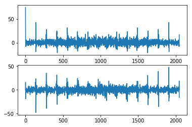
sample_size = 2048 # sample size in minutes

import fft
spec = fft.transform(time[:sample_size],0)
This is the resulting spectrum, real and imaginary parts:
plt.figure(1)
plt.subplot(2,1,1)
plt.plot(np.real(spec))

plt.subplot(2,1,2)
plt.plot(np.imag(spec))
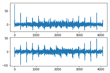
We now spread the spectrum to make it twice the size by simply adding a 0 at every second index. So a vector [1,2,3] would become [1,0,2,0,3,0].
The reason behind this is that after the inverse FFT the output signal will have twice the length in time-domain as compared to the input signal.
# spread spectrum to make it twice the size
spread = []
for s in spec:
    spread.extend([s,0])
The resulting spectrum looks identical, only the indices on the x-axis have changed:
plt.figure(1)
plt.subplot(2,1,1)
plt.plot(np.real(spread))

plt.subplot(2,1,2)
plt.plot(np.imag(spread))
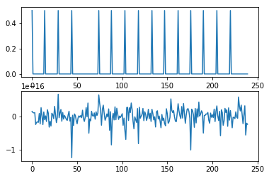
Perform inverse FFT
pred = fft.transform(spread,1)
pred = np.asarray(pred) / len(pred) # scaling
plt.figure(1)
plt.subplot(2,1,1)
plt.plot(np.real(pred[:240]))

plt.subplot(2,1,2)
plt.plot(np.imag(pred[:240]))
Now let’s compare the analyzed signal and how it continued with the signal after transformation and how FFT predicts it would continue:
plt.figure(1, figsize=[12,4])
plt.subplot(2,2,1)
plt.title("analyzed sample")
plt.plot(time[0:sample_size])
plt.subplot(2,2,2)
plt.title("how signal continues")
plt.plot(time[sample_size:(sample_size+2048)])

plt.subplot(2,2,3)
plt.title("sample after transformation")
plt.plot(np.abs(pred[0:sample_size]))
plt.subplot(2,2,4)
plt.title("predicted signal")
plt.plot(np.abs(pred[sample_size:(sample_size+2048)]))

plt.subplots_adjust(hspace=0.5)
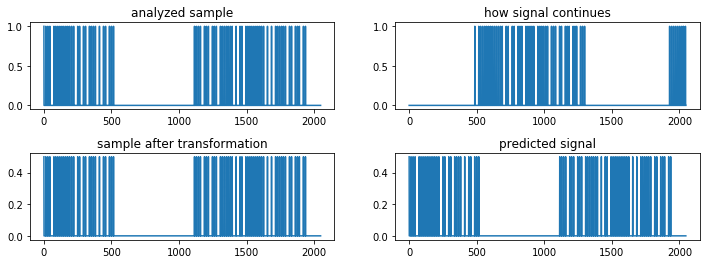
We see that the FFT just caused the same signal to be repeated a second time. This is not what we were hoping for. We were hoping that by calculating the signal from its frequency components we would get a good approximation to how the signal could continue.
Why didn’t it work?
The reason why the input signal is repeated a second time lies in the way how the discrete Fourier transform (DFT) works.
Remember, the DFT is defined as follows:
\(\displaystyle X(k)=\sum_{t=0}^{n-1} x(t) e^{-2 π i \frac{k}{n} t}\)Where \(X\) is the frequency component \(k\) of the discrete signal \(x(t)\). Note, \(n\) is the length of the array \(x\) AND the length of \(X\).
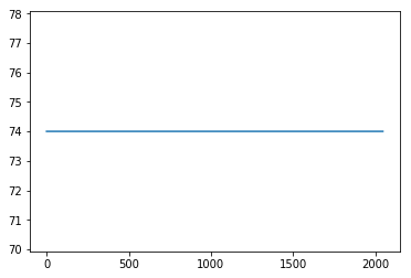
For example, let’s look at the frequency component \(X(0)\): For \(k=0\) the whole exponent vanishes and thus \(X(0)\) describes the constant component of \(x(t)\).
X0 = np.zeros(len(spec),dtype=complex)
X0[0]=spec[0]
signal = fft.transform(X0,1)
plt.figure(1)
plt.plot(np.abs(signal))
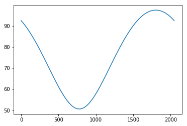
As next example, let’s look at \(X(1)\): The periodic part of the equation becomes \(e^{-2πi\frac{t}{n}}\), which is essentially exactly one sine wave over the whole range (0..n)
X1 = np.zeros(len(spec),dtype=complex)
X1[0]=spec[0]
X1[1]=spec[1]
signal = fft.transform(X1,1)
plt.figure(1)
plt.plot(np.abs(signal))
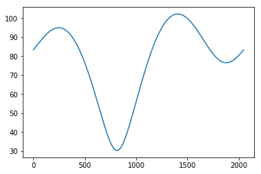
As last example, let’s look at \(X(2)\): The periodic part is \(e^{-2πi\frac{2t}{n}}\), which is a sine wave with doubled frequency as before. Overlaying the first 3 frequency components looks like this:
X2 = np.zeros(len(spec),dtype=complex)
X2[0]=spec[0]
X2[1]=spec[1]
X2[2]=spec[2]
signal = fft.transform(X2,1)
plt.figure(1)
plt.plot(np.abs(signal))
We see that the period of the frequency components is always an integer fraction of \(n\). This is no suprise because the index \(k\) in \(e^{-2πi\frac{k}{n}t}\) is always integer.
Thus, if we continued all frequency components outside of the transformed interval (\(t>n\)) the signal would exactly repeat itself.
I hope this short essay helps you understand, in case you have a similar idea to me. The idea might work if we didn’t do the discrete Fourier transformation but one that produces a continuous spectrum. That would also contain frequency components such as 1.5 and thus predict a different continuation of the signal. But I am not sure if that could be done with that kind of source data (list of timestamps of events).